Discrete differential geometry in homotopy type theory
\(\newcommand{\textesh}{∫}\) \(\newcommand{\ensuremath}{}\)
Abstract
Homotopy type theory captures all the major concepts of differential geometry including forms, connections, curvature, and gauge theory. We show this by focusing on combinatorial manifolds, which are discrete in the sense of real cohesion (Shulman, 2017a), and drawing inspiration from the similarly young field of discrete differential geometry.
“It is always ourselves we work on, whether we realize it or not. There is no other work to be done in the world.” — Stephen Talbott, The Future Does Not Compute (Talbott, 1995)
1 First introduction: homotopy type theory
For people trained in classical mathematics, as the author was, homotopy type theory (HoTT) is a major change of perspective. It is a new foundational system for mathematics which foregrounds fibrations and classifying spaces, and which defaults to a constructive philosophy. It is similar in those ways to the theory underpinning Lean and the formalization work happening in that community. But beyond that it also retains full fidelity of higher groupoidal structures and so supports homotopy theory directly in the syntax. The emphasis on syntax is quite alien to classical mathematicians, partially because that’s where the emphasis on foundations truly takes place, something workaday mathematicians don’t concern themselves with. This disorientation is acknowledged and soothed in perhaps the best starting point for HoTT for mathematicians, a survey by Mike Shulman (Shulman, 2017b).
The goal of this paper is to try to indicate just how much of differential geometry is emergent from the syntax of HoTT, making it a powerful new tool to prove theorems and generalize them to higher structures. For any differential geometer wishing to triangulate along with me between HoTT and geometry there is no better companion than Dan Freed and Mike Hopkins’ treatment of differential geometry through the lens of homotopy theory (Freed & Hopkins, 2013). Bringing all of their results into the HoTT framework would be a natural program that could follow from our discussion here.
2 Second introduction: discrete differential geometry
The observation that sparks the following discussion is this: if we can manage to reformulate differential geometry in discrete terms (i.e. finite, without infinitesimals) then we may also be able to construct it synthetically in homotopy type theory. Furthermore, if we do capture geometry in HoTT then there’s a chance that it can become clearer and smaller. We would then have new tools, a new audience, and a new program to (re)explore geometry, gauge theory, low dimensional topology, and mathematical physics.
Applied mathematicians and computer scientists have been developing discrete differential geometry (DDG) for many years. The 2003 Ph.D. thesis of Anil Hirani (Hirani, 2003) (see also the multi-author follow-up (Desbrun et al., 2005)) defines finite versions of vector fields, differential forms, the wedge product, the Hodge star, and several differential operators (exterior derivative, div, grad, curl, Laplace-Beltrami, Lie derivative). Hirani and others cite Whitney’s 1957 book Geometric Integration Theory (Whitney, 1957) which develops a theory of cochains by integrating smooth forms over chains. In 2004 Melvil Leok, Jerrold Marsden, and Alan Weinstein (Leok et al., 2005) defined discrete connections on principal bundles. This is probably the work most spiritually similar to this paper. The motivation for the above constructions was applied mathematics: modeling the differential equations of mechanics and fluid mechanics with the so-called “finite element” methods. The theory has been adopted and extended by the computer graphics community as well (see Keenan Crane’s course notes (Crane et al., 2013) for a gentle survey).
The applied category theory community has begun to develop category theoretic foundations and software libraries to increase the reusability and compositionality of finite element methods in science and engineering problems. See for example recent work to bring discrete exterior calculus into the AlgebraicJulia library (Morris et al., 2024) (Patterson et al., 2022).
For these classically-minded applied mathematicians DDG is defined on combinatorial manifolds such as simplicial complexes or polytopes, of any finite dimension. The 0-cells play the role of points, the 1-cells are path segments, and so on. They define \(n\)-forms as functions on the \(n\)-dimensional faces of the manifold into the real numbers, which is then extended by linearity to arbitrary \(n\)-chains. Exterior differentiation is defined by Stokes theorem (which is no longer a theorem in this setting), by which we mean the following.
Definition 1. (Exterior derivative in DDG.) Let \(\omega\) be an \(n-1\)-form on a combinatorial manifold \(M\), and let \(\Omega\) be an \(n\)-face of \(M\). Let \(\partial\) be the boundary operator on faces. The exterior derivative \(d\) is defined by \[d\omega(\Omega) = \omega(\partial\Omega).\]
At this point a study of DDG would move into chain complexes, where the forms of different dimensions are combined through the grading. Grassman algebras would be introduced, to convey the dependence of forms on orientation. The Leibniz rule (product rule) would be explored. Defining connections and curvature require constructing a codomain that is group-like and then creating more definitions about transport and holonomy. At that point major theorems like Gauss-Bonnet and Chern-Weil would be available to prove.
We will take a different path. We will not define forms, complexes, or Grassman algebras at all. We will view ordinary HoTT functions out of a type as synthetic discrete differential forms. The codomain will be a central H-space, which combines the features of the real numbers (in that functions can be pointwise multiplied) and classifying spaces of groups (so that maps into the H-space can classify bundles). We will then merely observe the emergence of various aspects of geometry.
We won’t be able to answer every question, so eventually we will stop and point to future directions.
3 Central H-spaces
Central H-spaces are the classifying spaces for principal bundles on abelian groups. We won’t be able to access the full theory for nonabelian groups just yet, but we hope that the theory of maximal tori and weights might bring even those within reach of the central H-space paradigm.
We will rely on the lovely paper by Buchholtz, Christensen, Flaten and Rijke (Buchholtz et al., 2023).
Definition 2. An H-space structure on a pointed type \((B,b)\) consists of
A binary operation \(\mu:B\to B\to B\)
A left unit law \(\mu_l:\mu(\mathrm{pt},-)=\ensuremath{\text{id}}_B\)
A right unit law \(\mu_r:\mu(-,\mathrm{pt})=\ensuremath{\text{id}}_B\)
A coherence \(\mu_{lr}:\mu_l(\mathrm{pt})=_{\mu(\mathrm{pt},\mathrm{pt})=\mathrm{pt}}\mu_r(\mathrm{pt})\)
A proof of left- and right- invertibility: \(\mu(a,-):A\simeq A\), \(\mu(-, b):A\simeq A\)
Proposition 1. ( (Buchholtz et al., 2023) Prop 3.6) Let \(A\) be a pointed type. Then the following are equivalent:
\(A\) is central.
\(A\) is a connected H-space and \(A\,\cdot\!\to A\) is a set.
\(A\) is a connected H-space and \(A\simeq A\) is a set.
This result will inform our study of the Leibniz rule: the analogue of the algebra of functions to \(\ensuremath{\mathbb{R}}\) is:
Proposition 2. For any type \(M\) and H-space \(B\) the type of maps \(M\to B\) with base point the constant map is an H-space under pointwise multiplication.
We will also be looking in detail at maps into the classifying space of \(S^1\) bundles. The Buchholtz et al paper (Buchholtz et al., 2023) describes this type in several helpful ways, summarized by:
Theorem 1. For any central H-space \(A\) (such as \(S^1\)) the type of torsors of \(A\) is a delooping of \(A\), and is equivalent to \(\mathrm{BAut}_1(S^1)\stackrel{\mathrm{def}}{=}\sum_{X:\mathcal{U}}||X=A||_0.\) This delooping is also a central H-space and so can be infinitely delooped.
This means that we can form a sequence of deloopings \(\ensuremath{\mathbb{Z}}, S^1, \mathrm{BAut}_1(S^1), \ldots\).
4 Higher maps contain connections
To hew close to the intended context of the term “connection” we will examine manifold-like types mapping into bundle-classifying-like types. The novelty here, compared to other HoTT investigations, is the focus on combinatorial types to stand in for manifolds.
In recent times it has been believed in the HoTT community that maps from a discrete type to a discrete classifying space can encode only the connections that a classical mathematician would call flat (zero curvature). In this context the word discrete means having the discrete topology, in the sense of cohesion (Shulman, 2017a). This is not the case! We will show that if the codomain is a classifying space of \(S^1\) or other group of homotopy dimension at least 1, then non-flat connections appear despite the type \(S^1\) being topologically discrete. Another common meaning of the shorthand “discrete” is to indicate a 0-truncated type, i.e. a set, as opposed to a type with higher homotopical structures. We will show that indeed if the codomain classifies sets, which is the case for example with the classifying space \(B\ensuremath{\mathbb{Z}}\), the delooping of \(\ensuremath{\mathbb{Z}}\), then connections are flat. (The type we denote by \(\mathbb{S}^1\stackrel{\mathrm{def}}{=}\{(x, y)|x^2+y^2=1\}\) is a set and is not topologically discrete. We will not be discussing it at all in this paper.)
The DDG philosophy tells us to look at HITs that are polytope-like. A polytope \(M\) will have finitely many 0-dimesional (point) constructors \(\{m_0^i\}\), finitely many 1-dimesnional constructors \(\{m_1^{ij}:m_0^i=m_0^j\}\), and so on. Type families \(f:M\to \mathcal{U}\) on this type specify where each of these constructors is sent. In DDG parlance, \(f\) restricted to the 0-dimensional constructors of \(M\) is a 0-form and \(f\) restricted to the 1-dimensional constructors (not the 1-skeleton but just the 1-dimensional parts, whatever that means in HoTT) is a 1-form, and so on.
A principal \(S^1\) bundle is a family of \(S^1\) torsors and so we will often be focusing on the function type \(M\to \mathrm{BAut}_1(S^1)\). The novel claim here is that \(M\to \mathrm{BAut}_1(S^1)\) contains more than just all the principal \(S^1\)-bundles: it also contains all the connections on all the bundles. Every connection is present, both curved and flat, because we have complete freedom to specify the images of the paths.
Classically, curvature is a property of the connection. It is computed either on infinitesimal loops, or on the infinitesimal surface bounded by the loop. In fact it is “the derivative of the connection” morally speaking. Getting into the details would wreck the simplicity we’re going for1. We will look for curvature by examining \(f\) on 1-dimensional loops. If \(M\) is at least a 2-type and if we want to claim that \(f\) classifies a bundle with connection, then we will be required to map the 2-faces of \(M\) (the 2-dimesional constructors) to a path from \(\ensuremath{\mathsf{refl}}\) to the image of a bounding loop. So at dimension 2 we will impose that constraint. Since \(\mathrm{BAut}_1(S^1)\) is 2-truncated, \(f\) factors through the truncation map \(M\to||M||_2\) and so that’s the top dimension.
There is an example at the end of this paper. For those who are best served by examples, do look at it and return to this point.
5 Why this is geometry
How can we double check that we are describing the intended theory of geometry? In this section we will enumerate a wishlist of facts that we believe characterize the subject, and then provide evidence for some of them.
Here are the translations that are covered in the current paper: \[\begin{aligned} & \text{\small Connections are infinitesimal splittings of a} & \quad &\text{\small Paths in a sigma type are equivalent to a} \\ & \text{\small principal bundle.} & \quad&\text{\small pair of paths.} \\ \hline & \text{\small Differentials satisfy the Leibniz (product) rule.} &\quad &\text{\small Horizontal composition in an H-space is} \\ & & \quad&\text{\small performed in two steps.} \\ \hline & \text{\small Connections with 0-truncated groups are covering} &\quad &\text{\small Transport around contractible loops is } \ensuremath{\mathsf{refl}}\\ & \text{\small spaces with unique flat connection.} & \quad&\text{\small when fibers are sets.} \\ \hline & \text{\small The group of gauge transformations (bundle} &\quad &\text{\small Homotopies of classifying maps respect } \\ & \text{\small automorphisms) acts on the space of connections.} & \quad&\text{\small the splitting of paths in sigma types.} \\ \end{aligned}\]
And here are questions to explore in the future:
There’s a notion of tensorial that holds for forms but not for connections.
Where is the Grassmannian structure of wedge product?
The Gauss-Bonnet theorem holds, relating the curvature of a 2-manifold to the Euler characteristic.
More generally, characteristic classes of bundles can be computed using a connection (Chern-Weil theory).
5.1 Connections as splittings
The classical story goes like this.
Definition 3. The vertical bundle \(VP\) of a principal bundle \(\pi:P\to M\) with Lie group \(G\) is the kernel of the derivative \(T\pi:TP\to TM\).
\(VP\) can be visualized as the collection of tangent vectors that point along the fibers. It should be clear that the group \(\mathrm{Aut}P\) acts on \(VP\): an automorphism \(\phi:P\to P\) sends \(V_pP\) to \(V_{\phi(p)}P\), where of course \(\pi(p)=\pi(\phi(p))\).
Definition 4. An Ehresmann connection on a principal bundle \(\pi:P\to M\) with Lie group \(G\) is a splitting \(TP=VP\oplus HP\) at every point of \(P\) into vertical and “horizontal” subspaces, which is preserved by the action of \(\mathrm{Aut}P\).
Being preserved by the action of \(\mathrm{Aut}P\) means that the complementary horizontal subspaces in a given fiber of \(\pi:P\to M\) are determined by the splitting at any single point in the fiber. The action of \(G\) on this fiber can then push the splitting around to all the other points.
The motivation for this definition is that we now have an isomorphism \(T_p\pi:H_pP\to T_{\pi(p)}M\) between each horizontal space and the tangent space below it in \(M\). This means that given a tangent vector at \(x:M\) and a point \(p\) in \(\pi^{-1}(x)\) we can uniquely lift the tangent vector to a horizontal vector at \(p\). We can also lift vector fields and paths in this way. To lift a path \(\gamma:[0,1]\to M\) you must specify a lift for \(\gamma(0)\) and then lift the tangent vectors of \(\gamma\) and prove that you can integrate the lift of that vector field upstairs in \(HP\).
Then, armed with the lifting of paths one immediately obtains isomorphisms between the fibers of \(P\). So the Ehresmann connection, the lifting of paths, and transport isomorphisms between fibers are all recapitulations of the structure that the connection adds to the bundle.
Moving now to HoTT, fix a type \(M:\mathcal{U}\) and a type family \(f:M\to\mathcal{U}\). Path induction gives us the transport isomorphism \(\prod_{p:x=_M y}\mathrm{tr}(p):f(x)=f(y)\). We can use this to define a type of dependent paths, also called pathovers or paths over a given path.
Definition 5. With the above context and points \(a:f(x), b:f(y)\) the type of dependent paths over \(p\) with endpoints \(a, b\) is denoted \[a\xrightarrow[{p}]{=}b.\] By induction we can assume \(p\) is \(\ensuremath{\mathsf{refl}}_a\) in which case \(a\xrightarrow[{p}]{=}b\) is \(a=_{f(x)}a\).
See (Bezem et al., 2023) for more discussion of dependent paths (where they use the term “path over”), including composition, and associativity thereof.
We recall now the identity type of sigma types:
Theorem 2. (HoTT book Theorem 2.7.2 (Univalent Foundations Program, 2013)) If \(f:M\to \mathcal{U}\) is a type family and \(w,w':\sum_{x:M}f(x)\) then there is an equivalence \[\mathsf{split}:(w=w')\simeq \sum_{p:\ensuremath{\mathrm{pr}}_1(w)=_M\ensuremath{\mathrm{pr}}_1(w')} \left[\mathrm{tr}(p)(\ensuremath{\mathrm{pr}}_2(w))\right] = \ensuremath{\mathrm{pr}}_2(w').\]
In particular, given \(p:x=_M y\) and \(w:f(x)\) we have \(w\xrightarrow[{p}]{=}tr(p)(w)\simeq tr(p)(w)=_{f(y)}tr(p)(w)\) which has the term \(\ensuremath{\mathsf{refl}}\) which we can call “the horizontal lift of \(p\) starting at \(w\).” We can imitate the classical definition of a connection by defining \(\omega\stackrel{\mathrm{def}}{=}\ensuremath{\mathrm{pr}}_2\circ\mathsf{split}\), the projection onto the vertical component. And thus in HoTT we can see the equivalence of transport and lifting of paths into horizontal and vertical components.
5.2 The Leibniz (product) rule
The Leibniz rule for exterior differentiation states that if \(f, g:M\to \ensuremath{\mathbb{R}}\) are two smooth functions to the real numbers then \(d(fg) = fdg + gdf\). Here \(fg\) is the function formed by taking the pointwise product of \(f\) and \(g\). This is an interaction between multiplication in \(\ensuremath{\mathbb{R}}\) and the action on vectors of smooth functions (the 1-forms \(df\) and \(dg\)).
To examine this situation in HoTT we need type-theoretic functions \(f, g:M\to B\) from some type \(M\) to a central H-space \(B\). Let \(\mu:B\to B\to B\) be the H-space multiplication. How does \(\mu\) act on paths? Suppose we have \(a, a', b, b':B\) and \(p:a=_B a', q:b=_B b'\). Then we also have homotopies \(\mu(p, -):\mu(a, -)=_{B\to B}\mu(a', -)\) and \(\mu(-,q):\mu(-,b)=_{B\to B}\mu(-,b').\) Since \(\mu(a, -):B=B\) is an (unpointed) equivalence of \(B\), and similarly for \(\mu(b, -)\) and so on, this data assembles into the following diagram of higher groupoid morphisms:
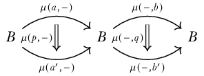
And so the two homotopies can be horizontally composed to give a path \[\mu(p,-)\star\mu(-,q): \mu(a, b)=\mu(a',b').\] Horizontal composition is given by \[\mu(p,-)\star\mu(-,q)\stackrel{\mathrm{def}}{=}(\mu(p,-)\cdot_r \mu(-,b))\cdot(\mu(a', -)\cdot_l\mu(-, q))\] where \[\mu(p,-)\cdot_r\mu(-,b):\mu(a,b)=\mu(a',b)\] and \[\mu(a',-)\cdot_l\mu(-,q):\mu(a',b)=\mu(a',b')\] are defined by path induction. See the HoTT book Theorem 2.1.6 on the Eckmann-Hilton argument (Univalent Foundations Program, 2013).
We can recognize the process of using whiskering to form horizontal composition in the Leibniz rule.
Quick aside: moving from infinitesimal calculus to finite groupoid algebra actually involves two changes. The first is the change from vectors to paths, forms to functions and so on. But it’s also the case that tangent vectors have just the one basepoint, whereas paths have two endpoints. You can see this play out in this example, where \(a\) and \(a'\) were distinct points (and \(b\) and \(b'\)).
The horizontal composition we build lives entirely in \(B\) and we didn’t make use of \(M\) yet. The Leibniz rule will be a pointwise version of what’s going on in \(B\). Denote by \(\mu\circ(f,g):B\to B\) the map which sends \(x\mapsto \mu(f(x),g(x))\).
Lemma 1. Given \(f, g:M\to B\) and \(p:x=_M y\) then \[\begin{aligned} \ensuremath{\mathsf{ap}}(\mu\circ(f,g))(p)&=\mu(f(p),-)\star\mu(-,g(p))\\ &=\left[\mu(f(p),-)\cdot_r \mu(-,g(x))\right]\cdot \left[\mu(f(y),-)\cdot_l\mu(-,g(p))\right]\\ &:\mu(f(x),g(x))=\mu(f(y),g(y)) \end{aligned}\]
5.3 Covering spaces
If \(G\) is a 0-truncated group such as \(\ensuremath{\mathbb{Z}}\) then the type of torsors (delooping) \(BG\) is 1-truncated. If \(f:M\to BG\) is a type family then \(\sum_{x:M}f(x)\) has fibers that are sets (\(G\)-torsors). So transport functions are set isomorphisms, and the transport of any contractible loop in \(M\) will be \(\ensuremath{\mathsf{refl}}\) (the identity) of the fiber, which is what we mean by flat.
5.4 Gauge transformations
A gauge transformation is a term inherited from physics. It’s an automorphism of a principal bundle \(P\to M\), meaning a homeomorphism of \(P\) that commutes with the projection to \(M\) and so acts on each fiber. It is further required to be equivariant under the action of the group \(G\), and so it’s very similar to the act of multiplying each fiber by a continuously varying element of \(G\).
In HoTT if the bundle is classified by \(f:M\to \mathcal{U}\) then an automorphism is a homotopy \(f\sim f\) and the group of gauge transformations is the loop space \(\Omega_f(M\to \mathcal{U})\).
Recall that torsors have a physical interpretation as a quantity without a specified unit, such as mass, length, or time. When we choose a base point in a torsor it becomes the standard torsor \(G\) acting on itself (for example, the additive real numbers). A physicist is looking for properties or laws that are independent of such a choice. In the 20th century physicists further wondered about choices of units that vary from point to point, and began searching for laws that are invariant under this much larger space of transformations. And so they and we are led to explore quotienting by the action of the group of gauge transformations, and in particular the space of connections “mod gauge.” In this scenario the base manifold \(M\) is spacetime, and a gauge transformation is a smoothly varying choice of gauge (units) at each point.
Gauge transformations act on connections. When we view connections as infinitesimal splittings of \(TP\) into vertical and horizontal sub-bundles, a gauge transformation that is constant in the neighborhood of a point will not change the splitting, it will just shift the fiber rigidly along itself, but one that is changing rapidly near a point will tilt the horizontal subspaces. So there are two effects: the effect of sliding along the fiber, and the effect of the rate of change of the gauge transformation. In classical geometry you’ll see formulas like this:
Theorem 3. Let \(P\to M\) be a principal bundle and \(A\in\Omega^1(M,\mathfrak{g})\) a connection 1-form on \(P\). Suppose that \(H\in \mathscr{G}(P)\) is a bundle automorphism. Then \(H^*A\) is a connection 1-form and in a neighborhood \(U\) of a point \(x\in M\) we can write \(H\) as a function \(H_U:U\to G\) where \(H_U(x)\in G\) is a group element multiplying the fiber at \(x\), and then we have \[H^*A=\mathrm{Ad}_{H_U(x)^{-1}}\circ A + H_U^*(\mu_G)\] where \(\mu_G:\Omega^1(G,\mathfrak{g})\) is the Maurer-Cartan form on \(G\).
This theorem is a combination of Theorems 5.2.2 and 5.4.4 in the excellent recent book on gauge theory for mathematicians interested in physics by Mark Hamilton (Hamilton, 2017).
It’s not so important to fully understand this formula because we will re-explain it in HoTT terms in a moment. But notice that \(H^*A\) (the action of the gauge transformation on the connection 1-form) has contributions from two terms (both of which are vertical — connections always map onto the vertical bundle). The first is the adjoint action at the specific point \(x\). This is always what we expect when we shift the base point in a torsor and look at the resulting group (or in this case, the Lie algebra). The second term involves the Maurer-Cartan form, which is the derivative of subtraction in the group. It takes tangent vectors at \(g:G\) to a tangent vector at the identity (the Lie algebra, denoted \(\mathfrak{g}\)) by differentiating the action of multiplication by \(g^{-1}\). If we think in terms of finite-length paths, then imagine a path \(p:g=g'\) and the function \((g^{-1}\cdot -)\). The function will act on the path to give a path \(g^{-1}\cdot p:e=(g'\cdot g^{-1})\) that starts at the identity. So the Maurer-Cartan form shifts paths to start at the identity by subtracting off the start point. Our Maurer-Cartan term is the pullback of the Maurer-Cartan form by \(H\) which records how \(H\) acts infinitesimally, i.e. the contribution from the gauge transformation \(H\) that comes from the rapidity of change from point to point. This term will be large when \(H_U\) has a large derivative.
In HoTT the connection’s parallel transport is visible as the transport function, and the horizontal-vertical splitting is visible in the decomposition of paths in the sigma type (total space) into pairs of paths. What is the effect of applying a homotopy \(H:f\sim f\) on transport, and on splitting?
\(H\) is a family of fiber automorphisms: \(H:\prod_{a:M}f(a)=f(a)\) which we can assemble into an equivalence \(H':\sum_{a:M}f(a)=\sum_{a:M}f(a)\) that acts fiberwise. We want to compute the action of \(\ensuremath{\mathsf{ap}}(H')\) on the horizontal-vertical decomposition of paths from Theorem 2 by computing \(\omega\circ\ensuremath{\mathsf{ap}}(H')=\ensuremath{\mathrm{pr}}_2\circ\mathsf{split}\circ\ensuremath{\mathsf{ap}}(H')\).
Denote \(\sum_{a:M}f(a)\) by \(P\). We’ll adopt a convention of roman letters for structures in \(M\) and Greek for those upstairs in \(P\). Let \(p:a=_M b\) be a path in the base and let \(\pi:(a,\alpha)=_P (b,\beta)\) be a path in \(P\) over \(p\). Then \(\omega(\pi):\mathrm{tr}_p(\alpha)=\beta\).
Now let’s apply \(H\). We have \(\ensuremath{\mathsf{ap}}(H')(\pi):(a,H(a)(\alpha))=_P(b,H(b)(\beta))\) which is still a path over \(p\). Applying \(\omega\) we get \[\omega(\ensuremath{\mathsf{ap}}(H')(\pi)):\mathrm{tr}_p(H(a)(\alpha))=(H(b)(\beta))\]. Using the lemma below we can if we wish rewrite this as \[\omega(\ensuremath{\mathsf{ap}}(H')(\pi)):H(b)\left[\mathrm{tr}_p(\alpha)=\beta\right]\] which uses only \(H(b)\).
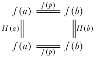
Lemma 2. Given a function \(f:M\to\mathcal{U}\) and homotopy \(H:f\sim f\) the following square commutes and so in the type family we have \(\mathrm{tr}(H(x)\cdot f(p)) = \mathrm{tr}(f(p)\cdot H(y))\).
5.5 Combinatorial manifolds
(This section is not quite off the ground.)
The combinatorial structure we have in mind is a nerve of a good open cover. What do we know about which smooth manifolds have such covers? While we’re at it, let’s survey all the combinatorial-flavored spaces and survey what smooth manifolds are homotopy equivalent to which structures.
What topological manifolds are equivalent to a CW complex? The answer is the composition of a few results summarized by Allen Hatcher2 (citing (Kirby & Siebenmann, 1977) and (Freedman & Quinn, 1990)):
Every topological manifold has a handlebody structure except in dimension 4, where a 4-manifold has a handlebody structure if and only if it is smoothable. This is a theorem on page 136 of Freedman and Quinn’s book “Topology of 4-Manifolds”, with a reference given to the Kirby-Siebenmann book for the higher-dimensional case. It is then an elementary fact that an \(n\)-manifold with a handlebody structure is homotopy equivalent to a CW complex with one \(k\)-cell for each \(k\)-handle, so in particular there are no cells of dimension greater than \(n\). At least in the compact case a manifold with a handlebody structure is in fact homeomorphic to a CW complex with \(k\)-cells corresponding to \(k\)-handles; see page 107 of Kirby-Siebenmann. This probably holds in the noncompact case as well, though I don’t know a reference.
6 Appendix: the tangent bundle of the 2-sphere
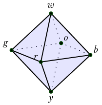
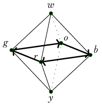
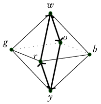
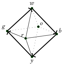
The usual HoTT \(S^1\) and \(S^2\) are a little impoverished, and seeing connections and curvature is difficult. Instead we will define equivalent HITs that have more constructors. The representation of the sphere will be the octohedron \(\ensuremath{\mathbb{O}}\) and the circle will be \(C_4\) which has four points and is designed to work well with \(\ensuremath{\mathbb{O}}\).
The Rubik’s cube has a convenient standardized arrangement of colors that start with different letters (white, yellow, blue, orange, green, red) so we will use those to label our points, especially since having such a cube handy is very helpful to visualize some of the geometry that is encoded below as mere lists of data.
Should the 0-dimensional constructors represent the corners or the faces? We have so far found it intuitive to imagine taking the nerve of a good open cover, where the top-dimensional bulk of the cube, namely the faces, is converted to a point since an open set covering that face is contractible. That’s why we end up with an icosohedron, which is a dual polyhedron to the cube.
We won’t discuss in detail the fact that Mike Shulman’s shape operator (Shulman, 2017a) is equivalent to taking the nerve of an open cover and forming a HIT from the overlap data. The shape operator preserves colimits and so the simple homotopy pushouts we are considering should be within the use cases of shape.
The HIT \(\ensuremath{\mathbb{O}}\) is built from the following constructors:
Dimension 0: the vertices \(\{w, y, b, g, r, o, y\}\) where we think of \(w\) as the north pole and \(y\) the south pole.
Dimension 1: the 12 adjacency pairs of faces, denoted \(\{wb\}, \{wo\}\) and so on.
Dimension 2: the set of faces generated by the 3-way adjacency of faces (which takes place in neighborhoods of the cube’s original corners), denoted \(\{wbo\}, \{wog\}\) and so on.
We will choose a base point of \(\mathrm{BAut}_1(S^1)\) that has four points, just like the equator of \(\ensuremath{\mathbb{O}}\).
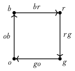
Definition 6. Denote by \(C_4\) the join \(\{b, g\}*\{r, o\}\). This is the equator of the discrete octahedral sphere. Then \(\ensuremath{\mathbb{O}}\) itself can be seen as the join \(\{w, y\}* C_4\).
Lemma 3. \((C_4, b)\simeq S^1\).
Proof. Similar to Lemma 6.5.1 from the HoTT book (Univalent Foundations Program, 2013). We will make some use of the particular map \(\{b, r, g, o\}\mapsto \mathsf{base}, br\mapsto \mathsf{loop}, \{rg, go, ob\}\mapsto \ensuremath{\mathsf{refl}}.\) ◻
Lemma 4. \(\ensuremath{\mathbb{O}}\simeq S^2\).
Proof. \(\ensuremath{\mathbb{O}}\) is the join of \(C_4\) and a two-point type. For more discussion of the join operation see the HoTT book section 8.5 (Univalent Foundations Program, 2013). ◻
To produce a term in \(\mathrm{BAut}_1(S^1)\) we need \(C_4\) and a choice of an equivalence class of equivalences with \(S^1\):
Lemma 5. We have \((C_4, ||\{b, r, g, o\}\mapsto \mathsf{base}, br\mapsto \mathsf{loop}, \{rg, go, ob\}\mapsto \ensuremath{\mathsf{refl}}||_0):\mathrm{BAut}_1(S^1)\)
There are other near-to-hand terms of \(\mathrm{BAut}_1(S^1)\) we can denote like: \([w, o, y, r]\), meaning the square isomorphic to \(C_4\) but with the given four points, with pointing given by whichever point we listed first, and with equivalence with \(S^1\) chosen so that the path between the first two points maps to \(\mathsf{loop}\). We will also introduce notation for maps \(f:[a, b, c, d]\to [w, x, y, z]\) by indicating where each item in the domain list is sent, like so: \(f\stackrel{\mathrm{def}}{=}[[x, y, z, w]]\).
\(C_4\) has an unpointed automorphism connected to the identiy which will play the role of rotation by 90 degrees:
Definition 7. Let \(R:C_4\to C_4\) be the cyclic permutation given by \(R(b)=r, R(r)=g, R(g)=o, R(o)=b, R(br)=rg, R(rg)=go, R(go)=ob, R(ob)=br.\) Let \(R':R=\ensuremath{\text{id}}\) be the obvious homotopy to the identity.
To construct a map \(\ensuremath{\mathbb{O}}\to\mathrm{BAut}_1(S^1)\) we need to send each vertex to an \(S^1\)-torsor such as \(C_4\). We will choose to send each vertex to “the clockwise equator if this was the north pole.”
Definition 8. Define \(T_0:\ensuremath{\mathbb{O}}\to\mathrm{BAut}_1(S^1)\) on just the 0-skeleton by
\(T_1(b)=[w, o, y, r]\).
\(T_1(o)=[w, g, y, b]\).
\(T_1(g)=[w, r, y, o]\).
\(T_1(r)=[w, b, y, g]\).
\(T_1(w)=[b, r, g, o]\).
\(T_1(y)=[b, o, g, r]\).
Extending this to the 1-skeleton requires various choices. We will choose the one that reflects the tangent bundle, using the transport we can intuitively see through the embedding of \(\ensuremath{\mathbb{O}}\) in 3-dimensional space as in our pictures. If you focus for a moment just on a path \(w\to b\to r\) and imagine rigidly tipping a moving equator along with a moving point, you can imagine a moving-equator point that starts at \(r\) and stays fixed when the north pole slides from \(w\) to \(b\). When the north pole continues sliding from \(b\) to \(r\) the moving-equator point moves to \(g\). Then it remains fixed when the north pole slides from \(r\) up to \(w\). So all in all we “moved \(r\) to \(g\).” When we track all the points on the original \(w\)-equator we see that we performed the rotation we earlier named \(R\).
In general we have:
Definition 9. Define \(T_1:\ensuremath{\mathbb{O}}\to\mathrm{BAut}_1(S^1)\) on just the 1-skeleton by extending \(T_0\) as follows: Transport away from \(w\):
\(T_1(wb):[b, r, g, o]\mapsto [y, r, w, o]\) (\(r, o\) fixed)
\(T_1(wr):[b, r, g, o]\mapsto [b, y, g, w]\) (\(b, g\) fixed)
\(T_1(wg):[b, r, g, o]\mapsto [w, r, y, o]\)
\(T_1(wo):[b, r, g, o]\mapsto [b, w, g, y]\)
Transport away from \(y\):
\(T_1(yb):[b, o, g, r]\mapsto [w, o, y, r]\)
\(T_1(yr):[b, o, g, r]\mapsto [b, y, g, w]\)
\(T_1(yg):[b, o, g, r]\mapsto [y, o, w, r]\)
\(T_1(yo):[b, o, g, r]\mapsto [b, w, g, y]\)
Transport along the equator:
\(T_1(br):[w, o, y, r]\mapsto [w, b, y, g]\)
\(T_1(rg):[w, b, y, g]\mapsto [w, r, y, o]\)
\(T_1(go):[w, r, y, o]\mapsto [w, g, y, b]\)
\(T_1(ob):[w, g, y, b]\mapsto [w, o, y, r]\)
At this point we have defined a map on the 1-skeleton of \(\ensuremath{\mathbb{O}}\).
Claim 1. \(T_1\) defines a principal circle bundle with connection over the 1-skeleton of \(\ensuremath{\mathbb{O}}\).
We now want to extend this map to all of \(\ensuremath{\mathbb{O}}\) by providing values for the eight faces. Here we will be guided by the classical relationship between a connection and its curvature. The curvature is computed from the connection, it doesn’t contain any new data. Classically the integral of curvature over a 2-cell is the holonomy given by transport around the boundary.
Definition 10. Define \(T_2:\ensuremath{\mathbb{O}}\to\mathrm{BAut}_1(S^1)\) by extending \(T_1\) as follows. We will send every clockwise triangle to \(R'\), the homotopy from \(\ensuremath{\mathsf{refl}}\) to \(R\):
\(T_2(wbr)=R'\)
\(T_2(wrg)=R'\)
\(T_2(wgo)=R'\)
\(T_2(ybo)=R'\)
\(T_2(yrb)=R'\)
\(T_2(ygr)=R'\)
\(T_2(yog)=R'\)
\(T_2(ybo)=R'\)
I’m picking and choosing where to tell the story fully twice (see the next section) and where to simply look for motivation.↩︎
https://mathoverflow.net/questions/201944/topological-n-manifolds-have-the-homotopy-type-of-n-dimensional-cw-complexes↩︎